A couple of months ago Erika Johnson a Neuroscience Master’s student at the University of Alberta shared with me an interesting problem she’s been facing while conducting series of analysis in histological samples of brain tissue. The problem was an interesting yet simple challenge in the general field of image analysis. Before jumping into the specifics of the problem, Erika explained to me the core of her research.
In Erika’s words –multiple sclerosis is a crippling autoimmune disease of the brain and spinal cord in which the brain to attack itself. This leads to severe disabilities in movement, sensation, and even cognition.– she also explained that –when the brain attacks itself it creates a lesion, which is an area in which the cells are injured and inflammation is prevalent.– Erika also shared something that was quite surprising –you see, the cause of these lesions remains relatively unknown. However, abnormally high iron load has been observed in brains with multiple sclerosis, and that is something I’m investigating in my thesis–
I asked her if iron wasn’t a normal substance in the brain, to what she commented –well yeah, while iron is required for the healthy brain to function, when concentrations exceed a certain point it can cause inflammation and even become toxic to the brain cells.”
Erika explained that scientists do not yet understand where this excess iron comes from, and that being able to study how much extra iron is found in the brains of those with multiple sclerosis, is an important step to understanding more about this disease.
So what is the problem Erika was facing? Erika explained that –an example of determining iron concentrations and its cellular locations can be carried out through the use of a histological protocol that, through a set of chemical reactions, highlights in blue the presence of iron in samples human tissue. This protocol is called the Perl’s Prussian protocol.– You can see a couple of samples below:
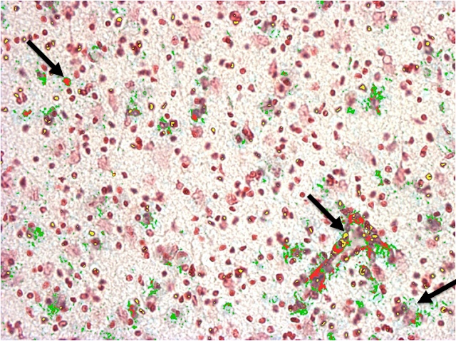
3. The analysis engine that I developed takes as input the images to be analyzed, along with the RGB values of the normative colors of each feature to be studied. In short the analysis engine analyses all the pixels of each image under study in order to identify and measure the areas where the normative colors are located, thus identifying and measuring the features of interest. The resulting process can be observed below. The color of each feature highlighter can be set up in the code.
In order to make the analysis engine more precise, the engine also receives as input two numbers that define the upper and a lower shade thresholds for each normative color assigned to a feature. This is, given that each feature may include multiple normative colors, and that each color may be found with different shade intensities in a feature, the shade thresholds help the engine to more precisely pinpoint the pixels corresponding to a feature regardless of the shade intensities of the normative colors present in its area.
Our experimental results revealed that using fine-tuned shade thresholds significantly improves the precision of the engine when identifying and measuring features. Furthermore, our implementation has a negligible feature intersection value. This is, in our empirical validation the total percentage of pixels that were assigned to more than one feature was 0.0069% on average across all the analyzed pictures.
4. Finally, once the areas of the features have been identified and measured in terms of their number of pixels, information such as the corresponding percentage our of the total picture size, and relations between feature sizes can be exported in plain textual files for further analysis. The reporting of the measurements was also a very interesting challenge to solve given how pathologist label and store the images of a sample and how each sample is split in multiple images. I’ll be sharing a a post on this matter soon!
The code is open source and it is available in github: https://github.com/guana/coloranalysis
Source: V.G. – RSS


No Comments